Monte Carlo simulation
Monte Carlo simulation
Our goal is to estimate our profit \(P\) based on the following variable
\(V\) - volume of production (number of produced units)
\(p\) - price of one unit
\(fc\) - fixed cost
\(vc\) - variable cost
using the formula \(P = V\cdot (p-vc)-fc\).
For each variable, we have received three estimation - minimum, best guess and maximum:
\(V=(10\,000; 40\, 000; 100\,000)\)
\(p=(100; 110; 150)\)
\(fc=(140\,000; 300\, 000; 420\,000)\)
\(vc=(10; 30; 105)\)
For the calculation we will use Monte Carlo simulation method and we will use triangular probability distribution.
%number of simulation
n=10000000
%Firstly, we will construct individual probability distributions
%probability distribution (pd) of Volume
V_pd = makedist('Triangular','A',10000,'B',40000,'C',100000);
%probability distribution (pd) of Price
p_pd = makedist('Triangular','A',100,'B',110,'C',150);
%probability distribution (pd) of Fixed cost
fc_pd = makedist('Triangular','A',140000,'B',300000,'C',420000);
%probability distribution (pd) of variable cost
vc_pd = makedist('Triangular','A',10,'B',30,'C',105);
%to obtain n random values of volume, we will use
V=random(V_pd,1,n);
%similar approach will be applied on remaining variables
p=random(p_pd,1,n);
fc=random(fc_pd,1,n);
vc=random(vc_pd,1,n);
%we will apply the whole formula to obtain n possible results
P=p.*(V-vc)-fc;
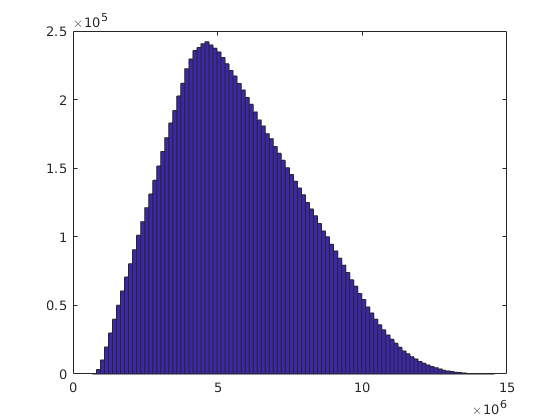
%and we will plot the results
hist(P,100)
xlim([0,15000000]);
n =

    10000000
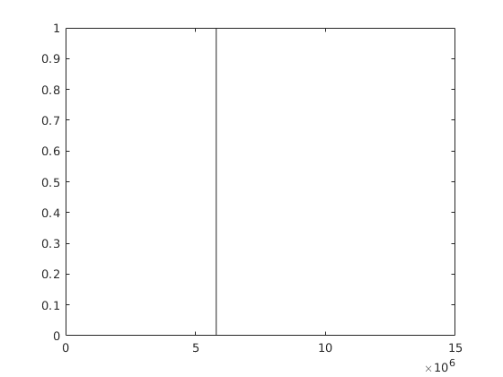
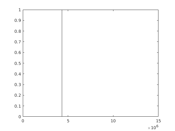
Lets make a deeper look into the computation. What will happen, if we do only one simulation?
n=1

%to obtain n random values of volume, we will use
V=random(V_pd,1,n);

%similar approach will be applied on remaining variables
p=random(p_pd,1,n);
fc=random(fc_pd,1,n);
vc=random(vc_pd,1,n);

%we will apply the whole formula to obtain n possible results
P=p.*(V-vc)-fc;

%and we will plot the results
hist(P,100)
xlim([0,15000000]);
n =

     1
And again
%to obtain n random values of volume, we will use
V=random(V_pd,1,n);

%similar approach will be applied on remaining variables
p=random(p_pd,1,n);
fc=random(fc_pd,1,n);
vc=random(vc_pd,1,n);

%we will apply the whole formula to obtain n possible results
P=p.*(V-vc)-fc;

%and we will plot the results
hist(P,100)
xlim([0,15000000]);
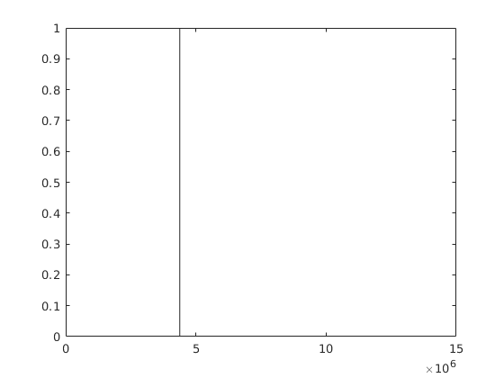
and again
n=1

%to obtain n random values of volume, we will use
V=random(V_pd,1,n);

%similar approach will be applied on remaining variables
p=random(p_pd,1,n);
fc=random(fc_pd,1,n);
vc=random(vc_pd,1,n);

%we will apply the whole formula to obtain n possible results
P=p.*(V-vc)-fc;

%and we will plot the results
hist(P,100)
xlim([0,15000000]);
n =

     1
As we can see, the output is random. Lets try 100 simulations
n=100

%to obtain n random values of volume, we will use
V=random(V_pd,1,n);

%similar approach will be applied on remaining variables
p=random(p_pd,1,n);
fc=random(fc_pd,1,n);
vc=random(vc_pd,1,n);

%we will apply the whole formula to obtain n possible results
P=p.*(V-vc)-fc;

%and we will plot the results
hist(P,100)
xlim([0,15000000]);
n =

   100
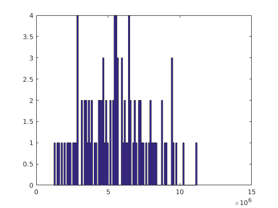
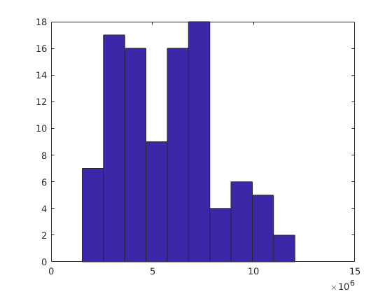
This is closer to the expected distribution - lets change the number of bins in histogram to 10
n=100

%to obtain n random values of volume, we will use
V=random(V_pd,1,n);

%similar approach will be applied on remaining variables
p=random(p_pd,1,n);
fc=random(fc_pd,1,n);
vc=random(vc_pd,1,n);

%we will apply the whole formula to obtain n possible results
P=p.*(V-vc)-fc;

%and we will plot the results
hist(P,10)
xlim([0,15000000]);
n =

   100